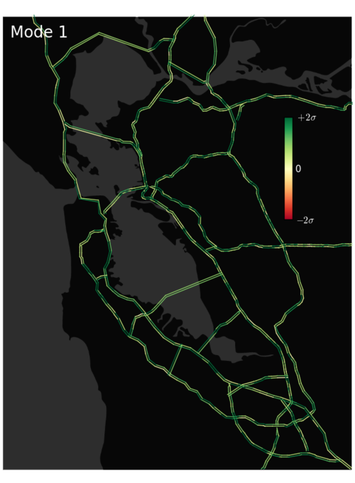
As we mentioned in the last post, there are currently over 2000 active speed loop detectors within the Bay Area highway system. The information provided by these loops is often highly redundant because speeds at neighboring sites typically differ little from one another. This observation suggests that a higher level, “macro” picture of traffic conditions could provide more insight: Rather than stating the speed at each detector, we might instead offer info like “101S is rather slow right now”. In fact, we aim to characterize traffic conditions as efficiently as possible. To move towards this goal, we have carried out a principal component analysis (PCA)\(^1\) of the full 2014 (year to date) PEMS data set.
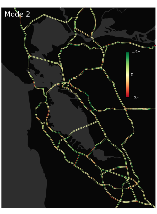
As described in [1] below, PCA provides us with a slick, automated method for identifying the most common “traffic patterns” or “modes” that get excited in our system. By adding together these patterns — with appropriate time-specific amplitudes — we can reconstruct the site-by-site traffic conditions observed at any particular moment. Importantly, summing over only the most significant modes will provide us with a system-tailored, minimal-loss method of data compression that will simplify our later prediction analysis. We will discuss this compression benefit further in the next post. Here, we present the two dominant modes of the Bay Area traffic system (see figures above). Notice that the first is fairly uniform, which presumably captures some nearly-site-independent changes in mean speed associated with night vs. daytime driving. In contrast, the second mode captures some interesting structure, showing slowdowns for some highways/directions and speedups for others. Evidently, this structure is the second most highly exhibited pattern in the Bay Area system; We couldn’t have intuited this pattern, but it has been captured automatically via our PCA.
[1] *Statistical physics of PCA: * One way of thinking about PCA as applied here is to imagine that the traffic system is harmonic. That is, we suppose that the traffic dynamics observed can be characterized by an energy cost function that is quadratic in the speeds of the different loops, measured relative to their average values, \(E = \frac{\beta^{-1}}{2} \delta \textbf{v}^{T} \cdot H \cdot \delta \textbf{v}.\) Here, \(\delta v_i = v_i - \langle v_i \rangle $ and $H\) is a matrix Hamiltonian. Under some effective, thermal driving, the pair correlation for two sites will be given by \(\langle \delta v_a \delta v_b \rangle \equiv
 Dustin got a B.S in Engineering Physics from the Colorado School of Mines (Golden, CO) before moving to UC Santa Barbara for graduate school. There he became interested in Soft Condensed Matter Physics and Polymer Physics, studying the interaction between single DNA molecules and salt ions. After a brief postdoc at UC San Diego studying the physics of bacterial growth, Dustin decided to move into the data science business for good - he is now a Quantitative Analyst at Google in Mountain View.