Stochastic geometric series

Let $a_1, a_2, \ldots$ be an infinite set of non-negative samples taken from a distribution $P_0(a)$, and write

$$\tag{1} \label{problem} S = 1 + a_1 + a_1 a_2 + a_1 a_2 a_3 + \ldots. $$

Notice that if the $a_i$ were all the same, $S$ would be a regular geometric series, with value $S = \frac{1}{1-a}$. How will the introduction of $a_i$ randomness change this sum? Will $S$ necessarily converge? How is $S$ distributed? In this post, we discuss some simple techniques to answer these questions.

Note: This post covers work done in collaboration with my aged p, S. Landy.

Introduction — a stock dividend problem

To motivate the sum (\ref{problem}), consider the problem of evaluating the total output of a stock that pays dividends each year in proportion to its present value — say $x %$. The price dynamics of a typical stock can be reasonably modeled as a geometric random walk$^1$:

$$\label{prod} \tag{2} price(t) = price(t-1) * a_t, $$

where $a_t$ is a random variable, having distribution $P_0(a_t)$. Assuming this form for our hypothetical stock, its total lifetime dividends output will be

$$\tag{3} x \times \sum_{t = 0}^{\infty} price(t) = x \times price(0) \left ( 1 + a_1 + a_1 a_2 + a_1 a_2 a_3 + \ldots \right) $$

The inner term in parentheses here is precisely (\ref{problem}). More generally, a series of this form will be of interest pretty much whenever geometric series are: Population growth problems, the length of a cylindrical bacterium at a series of time steps$^2$, etc. Will the nature of these sums change dramatically through the introduction of growth variance?

To characterize these types of stochastic geometric series, we will start below by considering their moments: This will allow us to determine the average value of (\ref{problem}), it’s variance etc. This approach will also allow us to determine a condition that is both necessary and sufficient for the sum’s convergence. Following this, we will introduce an integral equation satisfied by the $P(S)$ distribution. We demonstrate its application by solving the equation for a simple example.

The moments of $S$

To solve for the moments of $S$, we use a trick similar to that used to sum the regular geometric series: We write

$$\tag{4} \label{trick} S = 1 + a_1 + a_1 a_2 + \ldots \equiv 1 + a_1 T, $$

where $T = 1 + a_2 + a_2 a_3 + \ldots.$ Now, because we assume that the $a_i$ are independent, it follows that $a_1$ and $T$ are independent. Further, $S$ and $T$ are clearly distributed identically, since they take the same form. Subtracting $1$ from both sides of the above equation, these observations imply

$$\tag{5} \label{moments} \overline{(S-1)^k} = \sum_j {k \choose j} (-1)^j \overline{S^{k-j}} = \overline{ a^k S^k} = \overline{a^k} \ \overline{S^k}. $$

This expression can be used to relate the moments of $S$ to those of $a$ — a useful result, whenever the distribution of $a$ is known, allowing for the direct evaluation of its moments.

To illustrate, let us get the first couple of moments of $S$, using (\ref{moments}). Setting $k=1$ above, we obtain

$$\tag{6} \label{mean} \overline{S -1} = \overline{a} \overline{S} \ \ \to \ \ \overline{S} = \frac{1}{1 - \overline{a}} $$

The right side here looks just like the usual geometric sum result, with $a$ replaced by its average value. Similarly, setting $k =2$ in (\ref{moments}), we can solve for the second moment of $S$. Subtracting the square of the first gives the following expression for the sum’s variance,

$$\tag{7} \label{var} var(S) = \frac{var(a)}{(1 - \overline{a})^2(1 - \overline{a^2})}. $$

As one might intuit, the variance of $S$ is proportional to the variance of $a$.

Expressions (\ref{mean}) and (\ref{var}) are the most practical results of this post: They provide formal general expressions for the mean and variance for a sum of form (\ref{problem}). They can be used to provide a statistical estimate and error bar for a sum of form $S$ in any practical context. It is interesting/nice that the mean takes such a natural looking form — one that many people likely make use of already, without putting much thought into.

The expressions above are also of some theoretical interest: Note, for example, that as $\overline{a} \to 1$ from below, the average value of $S$ diverges, and then becomes negative as $a$ goes above this value. This is clearly impossible, as $S$ is a sum of positive terms. This indicates that $S$ has no first moment whenever $\overline{a} \geq 1$, while (\ref{mean}) holds whenever $\overline{a} < 1$. Similarly, (\ref{var}) indicates that the second moment of $S$ exists and is finite whenever $\overline{a^2} < 1$. In fact, this pattern continues for all $k$: $\overline{S^k}$ exists and is finite if and only if $\overline{a^k} < 1$ — a result that can be obtained from (\ref{moments}). A rigorous and elementary proof of these statements can be found in an earlier work by Szabados and Szekeley$^3$. The simple moment equation (\ref{moments}) can also be found there.

Condition for the convergence of $S$

A simple condition for the convergence of $S$ can also be obtained using (\ref{moments}). The trick is to consider the limit as $k$ goes to zero of the $k$-th moments. This gives, for example, the average of $1$ with respect to $P(S)$. If this is finite, then the distribution of $P$ is normalizable. Otherwise, $S$ must diverge: Setting $k = \epsilon$ in (\ref{moments}), expanding to first order in $\epsilon$ gives

$$\tag{8} \label{approximate_log} \overline{ \exp [\epsilon \log (S -1) ]} \sim \overline{ 1 + \epsilon \log (S -1) } \sim \overline{ 1 + \epsilon \log S } \ \overline{ 1 + \epsilon \log a}. $$

Solving for $\overline{1}_S$, the average of $1$ with respect to $P(S)$, gives

$$\tag{9} \overline{1}_S = \frac{\overline{\log( 1 - \frac{1}{S})}}{\log a} + O(\epsilon). $$

Like the integer moment expressions above, the right side here is finite up to the point where its denominator diverges. That is, the series will converge, if and only if $\overline{\log a} < 0$, a very simple condition$^4$.

Integral equation for the distribution $P(S)$

We have also found that one can sometimes go beyond solving for the moments of $S$, and instead solve directly for its full distribution: Integrating (\ref{trick}) over $a$ gives

\begin{eqnarray} \tag{10} \label{int} P(S_0) &=& \int da P_0(a) \int dS P(S) \delta(1+ a S - S_0) \\ &=& \int \frac{da}{a} P_0(a) P \left (\frac{S_0 -1}{a} \right). \end{eqnarray}

This is a general, linear integral equation for $P(S)$. At least in some cases, it can solved in closed-form. An example follows.

Uniformly distributed $a_i$

To demonstrate how one might solve the equation (\ref{int}), we consider here the case where the $a_i$ are uniform on $[0,1]$. In this case, writing $a = \frac{S_0 -1}{v}$, (\ref{int}) goes to

$$\tag{11} \label{int2} P(S_0) = \int_{S_0-1}^{\infty} P\left (v\right) \frac{1}{v}dv. $$

To progress, we differentiate with respect to $S_0$, which gives

$$\tag{12} \label{delay} P^{\prime} (S_0)\equiv - \frac{1 }{S_0 -1}\times P\left (S_0 -1\right). $$

Equation (\ref{delay}) is a delay differential equation. It can be solved through iterated integrations: To initiate the process, we note that $P(S_0)$ is equal to zero for all $S_0< 1$. Plugging this observation into (\ref{delay}) implies that $P(S_0) \equiv J$ — some constant — for $S \in (1,2)$. Continuing in this fashion, repeated integrations of (\ref{delay}) gives

$$\tag{13} P (S_0) = \begin{cases} J, \ \ \ S_0 \in (1,2) \\ J[1 - \log (S_0 -1)], \ \ \ S_0 \in (2,3) \\ J \left [ 1 - \log(S_0 - 1) + Li_2(2-S_0) + \frac{ \log(S_0 - 2)}{\log(S_0 - 1)} - Li_2(-1) \right ], \ \ S_0 \in (3,4) \\ \ldots, \end{cases} $$

where $Li_2$ is the polylogarithm function.

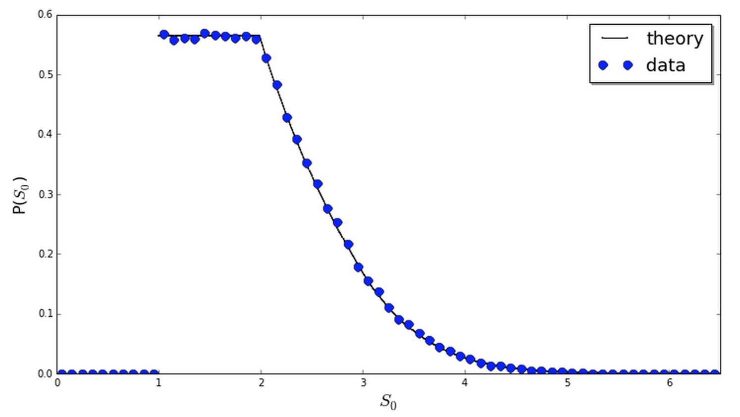
In practice, to find $J$ one can solve (\ref{delay}) numerically, requiring $P(S)$ to be normalized. The figure below compares the result to a simulation estimate, obtained via binning the results of 250,000 random sums of form (\ref{problem}). The two agree nicely.

Discussion

Consideration of this problem was motivated by a geometric series of type (\ref{problem}) that arose in my work at Square. In this case, I was interested in understanding the bias and variance in the natural estimate (\ref{mean}) to this problem. After some weeks of tinkering with S Landy, I was delighted to find that rigorous, simple results could be obtained to characterize these sums, the simplest being the moment and convergence results above. We now realize that these particular issues have already been well- (and better-)studied, by others$^3$.

As for the integral equation approach, we have not found any other works aimed at solving this problem in general. The method discussed in the example above can be used for any $P_0(a)$ that is uniform over a finite segment. We have also found solutions for a few other cases. Unfortunately, we have so far been unable to obtain a formal, general solution in closed form. However, we note that standard iterative approaches can always be used to estimate the solution to (\ref{int}). Finally, in cases where all moments exist, these can also be used to determine $P$.

References and comments

[1] For a discussion on the geometric random walk model for stocks, see here.

[2] Elongated bacteria — eg., e. coli — grow longer at an exponential rate — see my paper on how cell shape affects growth rates. Due to randomness inherent in the growth rates, bacteria populations will have a length distribution, similar in form to $P(S)$.

[3] “An exponential functional of random walks” by Szabados and Szekeley, Journal of Applied Probability 2003.

[4] Although we have given only a hand-waving argument for this result, the authors of [3] state — and give a reference for — the fact that it can be proven using the law of large numbers: By independence of the $a_i$, the $k$-th term in the series approaches $(\overline{\log a})^k$ with probability one, at large $k$. Simple convergence criteria then give the result.

[5] The moment equation (\ref{moments}) can also be obtained from the integral equation (\ref{int}), where it arrises from the application of the convolution theorem.

Jonathan Landy Jonathan grew up in the midwest and then went to school at Caltech and UCLA. Following this, he did two postdocs, one at UCSB and one at UC Berkeley. His academic research focused primarily on applications of statistical mechanics, but his professional passion has always been in the mastering, development, and practical application of slick math methods/tools. He currently works as a data-scientist at Stitch Fix.

Stochastic geometric series

Introduction — a stock dividend problem

The moments of \(S\)

Condition for the convergence of \(S\)

Integral equation for the distribution \(P(S)\)

Discussion

References and comments

Published

Category

Tags

Contact