Dynamic programming in reinforcement learning

Background

We discuss how to use dynamic programming (DP) to solve reinforcement learning (RL) problems where we have a perfect model of the environment. DP is a general approach to solving problems by breaking them into subproblems that can be solved separately, cached, then combined to solve the overall problem.

We’ll use a toy model, taken from [1], of a student transitioning between five states in college, which we also used in our introduction to RL:

student MDP

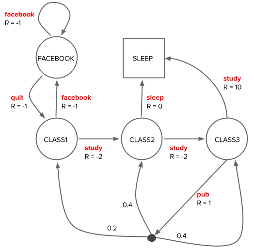
The model (dynamics) of the environment describe the probabilities of receiving a reward \(r\) in the next state \(s'\) given the current state \(s\) and action \(a\) taken, \(p(s’, r | s, a)\). We can read these dynamics off the diagram of the student Markov Decision Process (MDP), for example:

\(p(s'=\text{CLASS2}, r=-2 | s=\text{CLASS1}, a=\text{study}) = 1.0\)

\(p(s'=\text{CLASS2}, r=1 | s=\text{CLASS3}, a=\text{pub}) = 0.4\)

If you’d like to jump straight to code, see this jupyter notebook.

The role of value functions in RL

The agent’s (student’s) policy maps states to actions, \(\pi(a|s) := p(a|s)\). The goal is to find the optimal policy \(\pi_*\) that will maximize the expected cumulative rewards, the discounted return \(G_t\), in each state \(s\).

The value functions, \(v_{\pi}(s)\) and \(q_{\pi}(s, a)\), in MDPs formalize this goal.

\begin{eqnarray} v_{\pi}(s) &=& \mathbb{E}_{\pi}[G_t | S_t = s] \\ q_{\pi}(s, a) &=& \mathbb{E}_{\pi}[G_t | S_t = s, A_t = a] \end{eqnarray}

We want to be able to calculate the value function for an arbitrary policy, i.e. prediction, as well as use the value functions to find an optimal policy, i.e. the control problem.

Policy evaluation

Policy evaluation deals with the problem of calculating the value function for some arbitrary policy. In our introduction to RL post, we showed that the value functions obey self-consistent, recursive relations, that make them amenable to DP approaches given a model of the environment.

These recursive relations are the Bellman expectation equations, which write the value of each state in terms of an average over the values of its successor / neighboring states, along with the expected reward along the way.

The Bellman expectation equation for \(v_{\pi}(s)\) is

\begin{eqnarray}\label{state-value-bellman} \tag{1} v_{\pi}(s) = \sum_{a} \pi(a|s) \sum_{s’, r} p(s’, r | s, a) [r + \gamma v_{\pi}(s’) ], \end{eqnarray}

where \(\gamma\) is the discount factor \(0 \leq \gamma \leq 1\) that weights the importance of future vs. current returns. DP turns (\ref{state-value-bellman}) into an update rule (\ref{policy-evaluation}), \(\{v_k(s’)\} \rightarrow v_{k+1}(s)\), which iteratively converges towards the solution, \(v_\pi(s)\), for (\ref{state-value-bellman}):

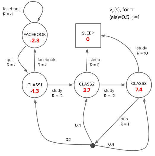
\begin{eqnarray}\label{policy-evaluation} \tag{2} v_{k+1}(s) = \sum_{a} \pi(a|s) \sum_{s’, r} p(s’, r | s, a) [r + \gamma v_k(s’) ] \end{eqnarray}

Applying policy evaluation to our student model for an agent with a random policy, we arrive at the following state value function (see jupyter notebook for implementation):

student MDP value function random policy

Finding the optimal value functions and policy

Policy iteration

We can evaluate the value functions for a given policy by turning the Bellman expectation equation (\ref{state-value-bellman}) into an update equation with the iterative policy evaluation algorithm.

But how do we use value functions to achieve our end goal of finding an optimal policy that corresponds to the optimal value functions?

Imagine we know the value function for a policy. If taking the greedy action, corresponding to taking \(\text{arg} \max_a q_{\pi}(s,a)\), from any state in that policy is not consistent with that policy, or, equivalently, \(\max_a q_{\pi}(s,a) > v_\pi(s)\), then the policy is not optimal since we can improve the policy by taking the greedy action in that state and then onwards following the original policy.

The policy iteration algorithm involves taking turns calculating the value function for a policy (policy evaluation) and improving on the policy (policy improvement) by taking the greedy action in each state for that value function until converging to \(\pi_*\) and \(v_*\) (see [2] for pseudocode for policy iteration).

Value iteration

Unlike policy iteration, the value iteration algorithm does not require complete convergence of policy evaluation before policy improvement, and, in fact, makes use of just a single iteration of policy evaluation. Just as policy evaluation could be viewed as turning the Bellman expectation equation into an update, value iteration turns the Bellman optimality equation into an update.

In our previous post introducing RL using the student example, we saw that the optimal value functions are the solutions to the Bellman optimality equation, e.g. for the optimal state-value function:

\begin{eqnarray}\label{state-value-bellman-optimality} \tag{3} v_*(s) &=& \max_a q_{\pi*}(s, a) \\ &=& \max_a \mathbb{E} [R_{t+1} + \gamma v_*(S_{t+1}) | S_t = s, A_t = a] \\ &=& \max_a \sum_{s’, r} p(s’, r | s, a) [r + \gamma v_*(s’) ] \end{eqnarray}

As a DP update equation, (\ref{state-value-bellman-optimality}) becomes:

\begin{eqnarray}\label{value-iteration} \tag{4} v_{k+1}(s) = \max_a \sum_{s’, r} p(s’, r | s, a) [r + \gamma v_k(s’) ] \end{eqnarray}

Value iteration combines (truncated) policy evaluation with policy improvement in a single step; the state-value functions are updated with the averages of the value functions of the neighbor states that can occur from a greedy action, i.e. the action that maximizes the right hand side of (\ref{value-iteration}).

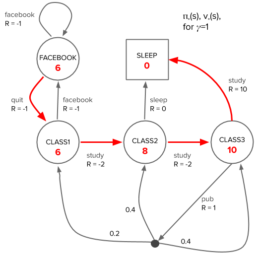
Applying value iteration to our student model, we arrive at the following optimal state value function, with the optimal policy delineated by red arrows (see jupyter notebook):

student MDP optimal policy and value function

Summary

We’ve discussed how to solve for (a) the value functions of an arbitrary policy, (b) the optimal value functions and optimal policy. Solving for (a) involves turning the Bellman expectation equations into an update, whereas (b) involves turning the Bellman optimality equations into an update. These algorithms are guaranteed to converge (see [1] for notes on how the contraction mapping theorem guarantees convergence).

You can see the application of both policy evaluation and value iteration to the student model problem in this jupyter notebook.

References

[1] David Silver’s RL Course Lecture 3 - Planning by Dynamic Programming (video, slides)

[2] Sutton and Barto - Reinforcement Learning: An Introduction - Chapter 4: Dynamic Programming

[3] Denny Britz’s notes on RL and DP, including crisp implementations in code of policy evaluation, policy iteration, and value iteration for the gridworld example discussed in [2].

[4] Deep RL Bootcamp Lecture 1: Motivation + Overview + Exact Solution Methods, by Pieter Abbeel (video, slides) - a very compressed intro.

Cathy Yeh Cathy Yeh got a PhD at UC Santa Barbara studying soft-matter/polymer physics. After stints in a translational modeling group at Pfizer in San Diego, Driver (a no longer extant startup trying to match cancer patients to clinical trials) in San Francisco, and Square, she is currently participating in the OpenAI Scholars program.