linselect demo: a tech sector stock analysis

This is a tutorial post relating to our python feature selection package, linselect. The package allows one to easily identify minimal, informative feature subsets within a given data set.

Here, we demonstrate linselect‘s basic API by exploring the relationship between the daily percentage lifts of 50 tech stocks over one trading year. We will be interested in identifying minimal stock subsets that can be used to predict the lifts of the others.

This is a demonstration walkthrough, with commentary and interpretation throughout. See the package docs folder for docstrings that succinctly detail the API.

Contents:

• Load the data and examine some stock traces
• FwdSelect, RevSelect; supervised, single target
• FwdSelect, RevSelect; supervised, multiple targets
• FwdSelect, RevSelect; unsupervised
• GenSelect

The data and a Jupyter notebook containing the code for this demo are available on our github, here.

The linselect package can be found on our github, here.

1 - Load the data and examine some stock traces

In this tutorial, we will explore using linselect to carry out various feature selection tasks on a prepared data set of daily percentage lifts for 50 of the largest tech stocks. This covers data from 2017-04-18 to 2018-04-13. In this section, we load the data and take a look at a couple of the stock traces that we will be studying.

Load data

The code snippet below loads the data and shows a small sample.

# load packages  
from linselect import FwdSelect, RevSelect, GenSelect  
import matplotlib.pyplot as plt  
import numpy as np  
import pandas as pd

# load the data, print out a sample  
df = pd.read_csv('stocks.csv')  
print df.iloc[:3, :5]  
print df.shape

# date AAPL ADBE ADP ADSK  
# 0 2017-04-18 -0.004442 -0.001385 0.000687 0.004884  
# 1 2017-04-19 -0.003683 0.003158 0.001374 0.017591  
# 2 2017-04-20 0.012511 0.009215 0.009503 0.005459  
# (248, 51)  

The last line here shows that there were 248 trading days in the range considered.

Plot some stock traces

The plot below shows Apple’s and Google’s daily lifts on top of each other, over our full date range (the code for the plot can be found in our notebook). Visually, it’s clear that the two are highly correlated — when one goes up or down, the other tends to as well. This suggests that it should be possible to get a good fit to any one of the stocks using the changes in each of the other stocks.

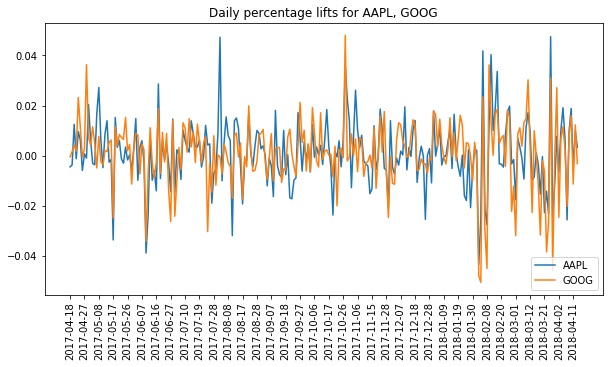
In general, a stock’s daily price change should be a function of the market at large, the behavior of its market segment(s) and sub-segment(s), and some idiosyncratic behavior special to the company in question. Given this intuition, it seems reasonable to expect one to be able to fit a given stock given the lifts from just a small subset of the other stocks — stocks representative of the sectors relevant to the stock in question. Adding multiple stocks from each segment shouldn’t provide much additional value since these should be redundant. We’ll confirm this intuition below and use linselect to identify these optimal subsets.

Lesson: The fluctuations of related stocks are often highly correlated. Below, we will be using linselect to find minimal subsets of the 50 stocks that we can use to develop good linear fits to one, multiple, or all of the others.

2 - FwdSelect and RevSelect; supervised, single target

Goal: Demonstrate how to identify subsets of the stocks that can be used to fit a given target stock well.

• First we carry out a FwdSelect fit to identify good choices.
• Next, we compare the FwdSelect and RevSelect results

Forward selection applied to AAPL

The code snippet below uses our forward selection class, FwdSelect to seek the best feature subsets to fit AAPL’s performance.

# Define X, y variables  
def get_feature_tickers(targets):  
    all_tickers = df.iloc[:, 1:].columns  
    return list(c for c in all_tickers if c not in targets)

TARGET_TICKERS = ['AAPL']  
FEATURE_TICKERS = get_feature_tickers(TARGET_TICKERS)

X = df[FEATURE_TICKERS].values  
y = df[TARGET_TICKERS].values

# Forward step-wise selection  
selector = FwdSelect()  
selector.fit(X, y)

# Print out main results of selection process (ordered feature indices, CODs)  
print selector.ordered_features[:3]  
print selector.ordered_cods[:3]

# [25, 7, 41]  
# [0.43813848, 0.54534304, 0.58577418]  

The last two lines above print out the main outputs of FwdSelect:

• The ordered_features list provides the indices of the features, ranked by the algorithm. The first index shown provides the best possible single feature fit to AAPL, the second index provides the next best addition, etc. Note that we can get the tickers corresponding to these indices using:
  python print [FEATURE_TICKERS[i] for i in selector.ordered_features[:3]] # ['MSFT' 'AVGO' 'TSM']
  A little thought plus a Google search rationalizes why these might be the top three predictors for AAPL: First, Microsoft is probably a good representative of the large-scale tech sector, and second the latter two companies work closely with Apple. AVGO (Qualcomm) made Apple’s modem chips until very recently, while TSM (Taiwan semi-conductor) makes the processors for iphones and ipads — and may perhaps soon also provide the CPUs for all Apple computers. Apparently, we can predict APPL performance using only a combination of (a) a read on the tech sector at large, plus (b) a bit of idiosyncratic information also present in APPL’s partner stocks.
• The ordered_cods list records the coefficient of determination (COD or R^2) of the fits in question — the first number gives the COD obtained with just MSFT, the second with MSFT and AVGO, etc.

A plot of the values in ordered_cods versus feature count is given below. Here, we have labeled the x-axis with the tickers corresponding to the elements of our selector.ordered_features. We see that the top three features almost fit AAPL’s performance as well as the full set!

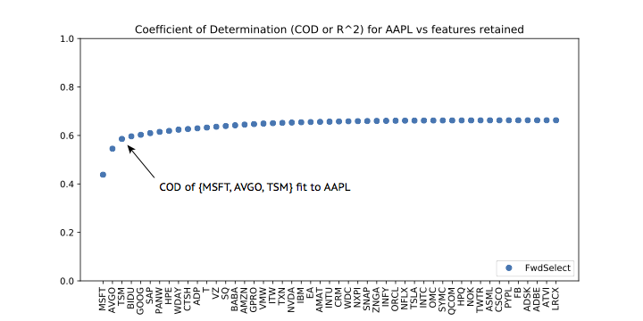
Lesson: We can often use linselect to significantly reduce the dimension of a given feature set, with minimal cost in performance. This can be used to compress a data set and can also improve our understanding of the problem considered.

Lesson: To get a feel for the effective number of useful features we have at hand, we can plot the output ordered_cods versus feature count.

Compare forward and reverse selection applied to TSLA

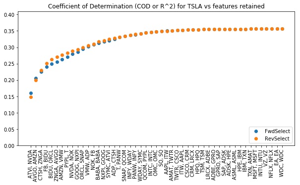
The code snippet below applies both FwdSelect and RevSelect to seek minimal subsets that fit Tesla’s daily lifts well. The outputs are plotted below this. This shows that FwdSelect performs slightly better when two or fewer features are included here, but that RevSelect finds better subsets after that.

Lesson: In general, we expect forward selection to work better when looking for small subsets and reverse selection to perform better at large subsets.

# Define X, y variables  
TARGET_TICKERS = ['TSLA']  
FEATURE_TICKERS = get_feature_tickers(TARGET_TICKERS)

X = df[FEATURE_TICKERS].values  
y = df[TARGET_TICKERS].values

# Forward step-wise selection  
selector = FwdSelect()  
selector.fit(X, y)

# Reverse step-wise selection  
selector2 = RevSelect()  
selector2.fit(X, y)  

3 - FwdSelect and RevSelect; supervised, multiple targets

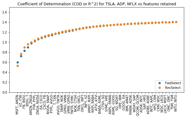
In the code below, we seek feature subsets that perform well when fitting multiple targets simultaneously.

Lesson: linselect can be used to find minimal feature subsets useful for fitting multiple targets. The optimal, “perfect score” COD in this case is equal to number of targets (three in our example).

# Define X, y variables  
TARGET_TICKERS = ['TSLA', 'ADP', 'NFLX']  
FEATURE_TICKERS = get_feature_tickers(TARGET_TICKERS)

X = df[FEATURE_TICKERS].values  
y = df[TARGET_TICKERS].values

# Forward step-wise selection  
selector = FwdSelect()  
selector.fit(X, y)

# Reverse step-wise selection  
selector2 = RevSelect()  
selector2.fit(X, y)  

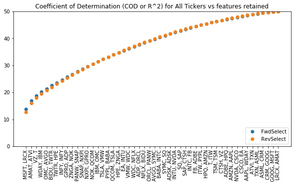
4 - FwdSelect and RevSelect; unsupervised

Here, we seek those features that give us a best fit to / linear representation of the whole set. This goal is analogous to that addressed by PCA, but is a feature selection variant: Whereas PCA returns a set of linear combinations of the original features, the approach here will return a subset of the original features. This has the benefit of leaving one with a feature subset that is interpretable.

(Note: See [1] for more examples like this. There, I show that if you try to fit smoothed versions of the stock performances, very good, small subsets can be found. Without smoothing, noise obscures this point).

Lesson: Unsupervised selection seeks to find those features that best describe the full data set — a feature selection analog of PCA.

Lesson: Again, a perfect COD score is equal to the number of targets. In the unsupervised case, this is also the number of features (50 in our example).

# Set X equal to full data set.  
ALL_TICKERS = list(df.iloc[:, 1:].columns)  
X = df[ALL_TICKERS].values

# Stepwise regressions  
selector = FwdSelect()  
selector.fit(X)

selector2 = RevSelect()  
selector2.fit(X)  

5 - GenSelect

GenSelect‘s API is designed to expose the full flexibility of the efficient linear stepwise algorithm. Because of this, its API is somewhat more complex than that of FwdSelect and RevSelect. Here, our aim is to quickly demo this API.

The Essential ingredients:

• We pass only a single data matrix X, and must specify which columns are the predictors and which are targets.
• Because we might sweep up and down, we cannot define an ordered_features list as in FwdSelect and RevSelect (the best subset of size three now may not contain the features in the best subset of size two). Instead, GenSelect maintains a dictionary best_results that stores information on the best results seen so far for each possible feature count. The keys of this dictionary correspond to the possible feature set sizes. The values are also dictionaries, each having two keys: s and cod. These specify the best feature subset seen so far with size equal to the outer key, and the corresponding COD, respectively.
• We can move back and forth, adding features to or removing them from the predictor set. We can specify the search protocol for doing this.
• We can reposition our search to any predictor set location and continue the search from there.
• We can access the costs of each possible move from our current location, without stepping.

If an \(m \times n\) data matrix X is passed to GenSelect, three Boolean arrays define the state of the search.

• s — This array specifies which of the columns are currently being used as predictors.
• targets — This specifies which of the columns are the target variables.
• mobile — This specifies which of the columns are locked into or out of our fit — those that are not mobile are marked False.

Note: We usually want the targets to not be mobile — though this is not the case in unsupervised applications. One might sometimes also want to lock certain features into the predictor set, and the mobile parameter can be used to accomplish this.

Use GenSelect to carry out a forward sweep for TSLA

The code below carries out a single forward sweep for TSLA. Note that the protocol argument of search is set to (1, 0), which gives a forward search (see docstrings). For this reason, our results match those of FwdSelect at this point.

Lesson: Setting up a basic GenSelect call requires defining a few input parameters.

# Define X  
X = df[ALL_TICKERS].values

# Define targets and mobile Boolean arrays  
TARGET_TICKERS = ['TSLA']  
FEATURE_TICKERS = get_feature_tickers(TARGET_TICKERS)  
targets = np.in1d(ALL_TICKERS, TARGET_TICKERS)  
mobile = np.in1d(ALL_TICKERS, FEATURE_TICKERS)

# Set up search with an initial \`position\`. Then search.  
selector = GenSelect()  
selector.position(X, mobile=mobile, targets=targets)  
selector.search(protocol=(1, 0), steps=X.shape[1])

# Review best 3 feature set found  
print np.array(ALL_TICKERS)[selector.best_results[3]['s']], selector.best_results[3]['cod']

# ['ATVI' 'AVGO' 'CTSH'] 0.225758  

Continue the search above

A GenSelect instance always retains a summary of the best results it has seen so far. This means that we can continue a search where we left off after a search call completes. Below, we reposition our search and sweep back and forth to better explore a particular region. Note that this slightly improves our result.

Lesson: We can carry out general search protocols using GenSelect‘s position and search methods.

# Reposition back to the best fit of size 3 seen above.  
s = selector.best_results[3]['s']  
selector.position(s=s)

# Now sweep back and forth around there a few times.  
STEPS = 10  
SWEEPS = 3

selector.search(protocol=(0, 1), steps=STEPS)  
selector.search(protocol=(2 * STEPS, 2 * STEPS), steps=SWEEPS * 4 * STEPS)

# Review best results found now with exactly N_RETAINED features (different from first pass in cell above?)  
print np.array(ALL_TICKERS)[selector.best_results[3]['s']], selector.best_results[3]['cod']

# ['AMZN' 'NVDA' 'ZNGA'] 0.229958  

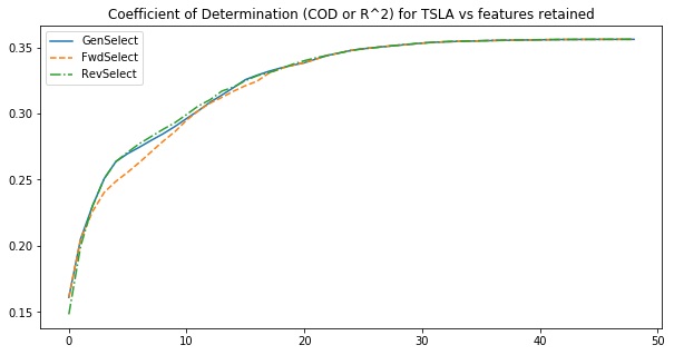
Compare to forward and reverse search results

Below, we compare the COD values of our three classes.

Lesson: GenSelect can be used to do a more thorough search than FwdSelect and RevSelect, and so can sometimes find better feature subsets.

# Get the best COD values seen for each feature set size from GenSelect search  
gen_select_cods = []  
for i in range(1, X.shape[1]):  
    if i not in selector.best_results:  
        break  
    gen_select_cods.append(selector.best_results[i]['cod'])

# Plot cod versus feature set size.  
fig, ax = plt.subplots(figsize=(10,5))  
plt.plot(gen_select_cods, label='GenSelect')

# FwdSelect again to get corresponding results.  
selector2 = FwdSelect()  
selector2.fit(X[:, mobile], X[:, targets])  
plt.plot(selector2.ordered_cods,'--', label='FwdSelect')

# RevSelect again to get corresponding results.  
selector3 = RevSelect()  
selector3.fit(X[:, mobile], X[:, targets])  
plt.plot(selector3.ordered_cods, '-.',label='RevSelect')  
plt.title('Coefficient of Determination (COD or R^2) for {target} vs features retained'.format(  
target=', '.join(TARGET_TICKERS)))  
plt.legend()  
plt.show()  

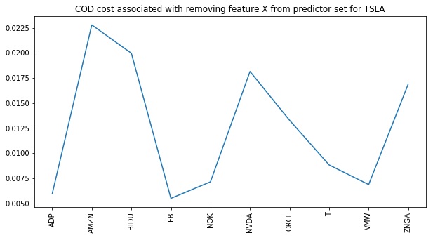
Examine the cost of removing a feature from the predictor set

Below, we reposition to the best feature set of size 10 seen so far. We then apply the method reverse_cods to expose the cost of removing each of these individuals from the predictor set at this point. Were we to take a reverse step, the feature with the least cost would be the one taken (looks like FB from the plot).

Lesson: We can easily access the costs associated with removing individual features from our current location. We can also access the COD gains associated with adding in new features by calling the forward_cods method.

# Reposition  
s = selector.best_results[10]['s']  
selector.position(s=s)

# Get costs to remove a feature (see also \`forward_cods\` method)  
costs = selector.reverse_cods()[s]  
TICKERS = np.array(ALL_TICKERS)[selector.best_results[10]['s']]

# Plot costs to remove each feature given current position  
fig, ax = plt.subplots(figsize=(10,5))  
plt.plot(costs)  
plt.xticks(np.arange(0, len(TICKERS)), rotation=90)  
ax.set_xticklabels(TICKERS)  
plt.show()  

Final comments

In this tutorial, we’ve illustrated many of the basic API calls available in linselect. In a future tutorial post, we plan to illustrate some interesting use cases of some of these API calls — e.g., how to use GenSelect‘s arguments to explore the value of supplemental features, added to an already existing data set.

References

[1] J. Landy. Stepwise regression for unsupervised learning, 2017. arxiv.1706.03265.

Like this post? Share on: Twitter | Facebook | Email

Jonathan Landy Jonathan grew up in the midwest and then went to school at Caltech and UCLA. Following this, he did two postdocs, one at UCSB and one at UC Berkeley.  His academic research focused primarily on applications of statistical mechanics, but his professional passion has always been in the mastering, development, and practical application of slick math methods/tools. He currently works as a data-scientist at Stitch Fix.