There were a number of upsets in the NBA this past Christmas week. Here, we offer no explanation, but do attempt to quantify just how bad those upsets were, taken in aggregate. Short answer: real bad! To argue this point, we review and then apply a very simple predictive model for sporting event outcomes — python code given in footnotes.
Quick review of x-mas week The Christmas holiday week\(^1\) (Dec. 19 - 25) provided a steady stream of frustrating upsets. The two most perplexing, perhaps, were the Lakers win over the Warriors and the Jazz win over the Grizzlies: two of this year’s greats losing to two of its most lackluster. In all, \(24\) of the \(49\) games that week were upsets (with an upset defined here to be one where the winning team started the game with a lower win percentage than the loser). That comes out to an upset ratio just under \(49%\), much higher than the typical rate, about \(34%\).
A general sporting model A \(49%\) upset rate sounds significant. However, this metric does not quite capture the emotional magnitude of the debacle. To move towards obtaining such a metric, we first review here a “standard”\(^2\) sporting model that will allow us to quantify the probability of observing a week as bad as this just past. For each team \(i\), we introduce a variable \(h_i\) called its mean scoring potential: Subtracting from this the analogous value for team \(j\) gives the expected number of points team \(i\) would win by, were it to play team \(j\). More formally, if we let the win-difference for any particular game be \(y_{ij}\), we have
where we average over hypothetical outcomes on the right in order to account for the variability characterizing each individual game.
By taking into account the games that have already occurred this season, one can estimate the set of \(\{h_i\}\) values. For example, summing the above equation over all past games played by team \(1\), we obtain
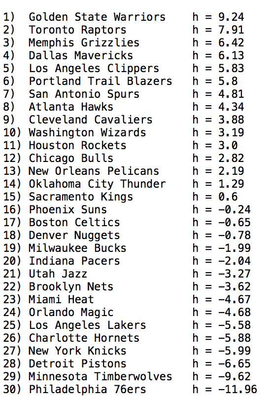
Here, in the sum on right we have approximated the averaged sum in the middle by the score differences actually observed in the games already played (note that in the sum on \(j\) here, each team appears exactly the number of times they have already played team \(1\) — this could be zero, once, twice, etc.) Writing down all equations analogous to this last one (one for each team) returns a system of \(30\) linear equations in the \(30\) \(\{h_i\}\) variables. This system can be easily solved using a computer\(^3\). We did this, applying the algorithm to the complete set of 2014-15 games played prior to the Christmas week, and obtained the set of \(h\) values shown at right\(^4\). The ranking looks quite reasonable, from top to bottom.
A Gaussian NBA Now that we have the \(\{h_i\}\) values, we can use them to estimate the mean score difference for any game. For example, in a Warriors-76ers game, we’d expect the Warriors to win, since they have the larger \(h\) value. Further, on average, we’d expect them to win by about \(h_{\text{War's}} - h_{\text{76's}}\) \( = 9.24 - (-11.96) \approx 21\) points. These two actually played this week, on Dec 30, and the Warriors won by \(40\), a much larger margin than predicted.
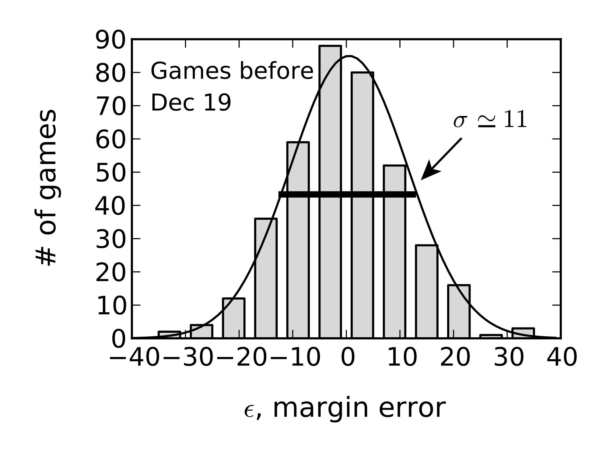
The distinction between our predicted and the actual Warriors-76ers outcome motivates further consideration of the variability characterizing NBA games. It turns out that if we analyze the complete set of games already played this year, something simple pops out: Plotting a histogram of our estimate errors, \(\epsilon_{ij} \equiv (h_i - h_j) - y_{ij}\), we see that the actual score difference distribution of NBA games looks a lot like a Gaussian, or bell curve. This is centered about our predicted value and has a standard deviation of \(\sigma \approx 11\) points, as shown in the figure at right. These observations allow us to estimate various quantities of interest. For instance, we can estimate the frequency with which the Warriors should beat the 76ers by 40 or more points, as they did this week. This is simply equal to the frequency with which we underestimate the winning margin by at least \(40 - 21 = 19\) points. This, in turn, can be estimated by counting how often this has already occurred in past games, using our histogram. Alternatively, we can use the fact that our errors are Gaussian distributed to write this as
where we have evaluated the integral by computer. This result says that a Warriors win by 40 or more points will only occur about \(4.2%\) of the time. Using a similar argument, one can show that the 76ers should beat the Warriors only about \(2.8 %\) of the time.
Christmas week, quantified It is now a simple matter to extend our analysis method so that we can estimate the joint likelihood of a given set of outcomes all happening the same week: We need only make use of the fact that the mean estimate error \(\langle \epsilon \rangle\) of our predictions on a set of \(N\) games \((\langle \epsilon \rangle = \frac{1}{N}\sum_{\text{games }i = 1}^N \epsilon_i)\) will also be Gaussian distributed, but now with standard deviation \(\sigma/ \sqrt{N}\). The \(1/\sqrt{N}\) factor here reduces the width of the mean error distribution, relative to that of the single games — it takes into account the significant cancellations that typically occur when you sum over many games, some with positive and some with negative errors. A typical week has about \(50\) games, so the mean error standard deviation will usually be about \(11/\sqrt{50} \approx 1.6\).
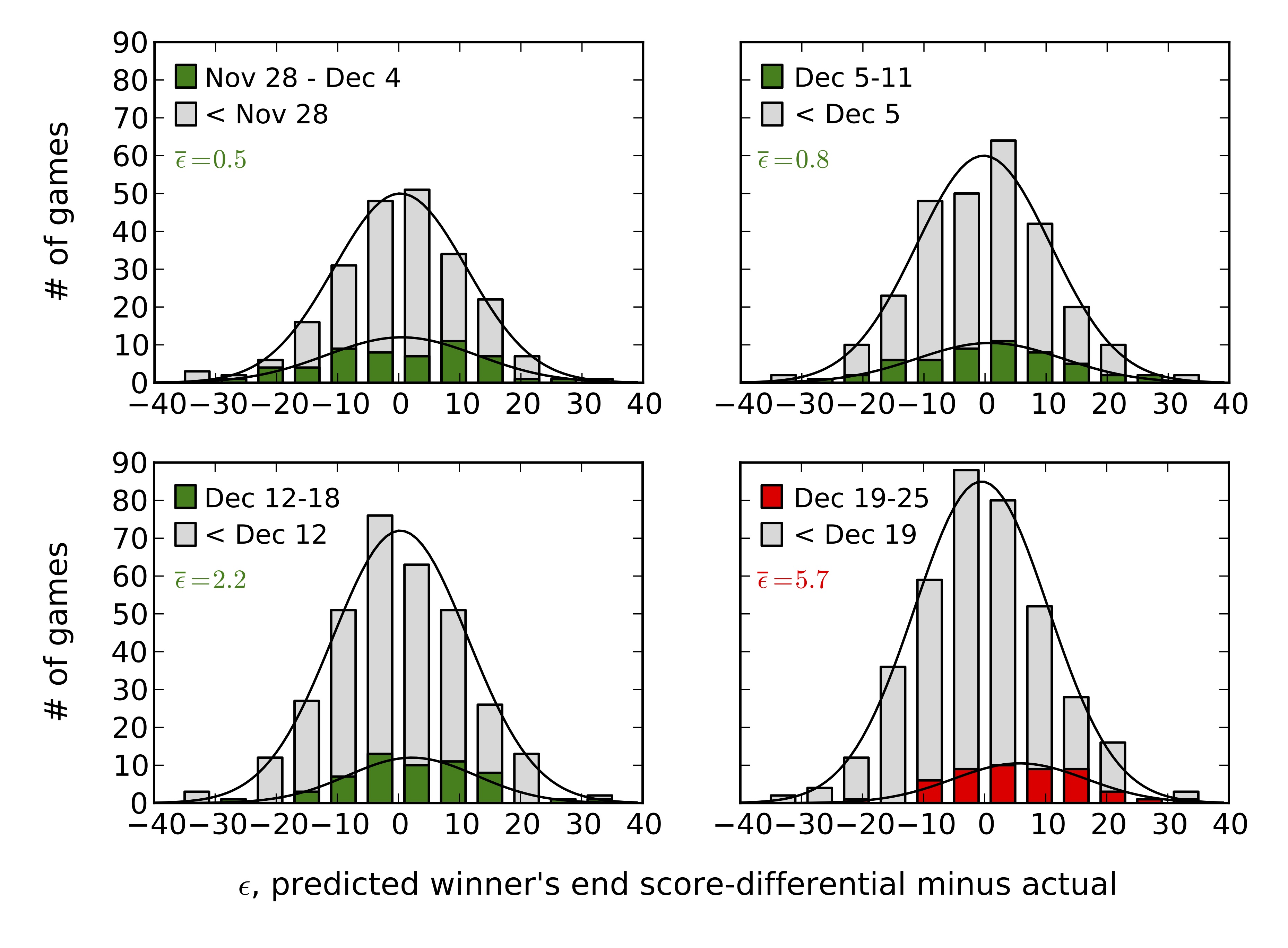
In the four figures below, we plot histograms of our prediction errors for four separate weeks: Christmas week is shown last (in red), and the other subplots correspond to the three weeks preceding it (each in green). We also show in each subplot (in gray) a histogram of all game errors preceding the week highlighted in that subplot — notice that each is quite well-fit by a Gaussian. In the first week, \(53\) games were played, and our average error on these games was just \(\langle \epsilon \rangle = 0.5\) points. The probability of observing an average overestimate of \(0.5\) or greater in such a week is given by,
That is, a weekly average overestimate of \(\langle \epsilon \rangle \geq 0.5\) will happen about \(38%\) of the time, and so is pretty common. Similarly, in the second, third, and fourth weeks, the number of games played and average estimate errors were \((N,\langle \epsilon \rangle) = (52,0.8),\) \((55,2.2)\), and \((49,5.7)\), respectively. Calculating as above, overestimates of these magnitudes or larger occur with frequency \(30%\), \(7%\), and \(0.01 %\), respectively. The previous two are both fairly common, but — on average — it would apparently take about ten thousand trials to find a week as bad as Christmas week 2014.
Discussion A week in ten thousand is equivalent to about one week in every \(400\) seasons! We don’t really take this estimate too seriously. In fact, we suspect that one of the following might be happening here: a) there may have been something peculiar about the games held this Christmas week that caused their outcomes to not be distributed in the same manner as other games this season\(^5\), b) alternatively, there may be long tails in the error distribution that we can’t easily observe, or c) it may be that improvements to our model (e.g., taking into account home team advantage, etc.) would result in a larger frequency estimate. Maybe all three are true, or maybe this really was a week in ten thousand. Either way, it’s clear that this past Christmas week was a singular one.
Footnotes [1] The NBA workweek starts on Friday.
[2] We first read about this modeling method here. In the addendum, it’s stated that the author thinks that nobody in particular is credited with having developed it, and that it’s been around for a long time.
[3] Notice that we can shift all \(h_i \to h_i +c\), with \(c\) some common constant. This invariance means that the solution obtained by solving the system of equations is not unique. Consequently, the matrix of coefficients is not invertible, and the system needs to be solved by Gaussian elimination, or some other irritating means.
[4] Python code and data for evaluating the NBA \(h\) values given here.
[5] Note, however, that carrying out a similar analysis over the past 9 seasons showed no similar anomalies in their respective Christmas weeks.
 Jonathan grew up in the midwest and then went to school at Caltech and UCLA. Following this, he did two postdocs, one at UCSB and one at UC Berkeley. His academic research focused primarily on applications of statistical mechanics, but his professional passion has always been in the mastering, development, and practical application of slick math methods/tools. He currently works as a data-scientist at Stitch Fix.