Two microphones are placed in a room where two conversations are taking place simultaneously. Given these two recordings, can one “remix” them in some prescribed way to isolate the individual conversations? Yes! In this post, we review one simple approach to solving this type of problem, Independent Component Analysis (ICA). We share an ipython document implementing ICA and link to a youtube video illustrating its application to audio de-mixing.
Introduction
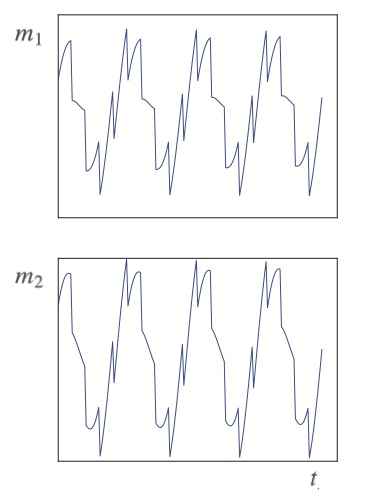
To formalize the problem posed in the abstract, let two desired conversation signals be represented by \(c_1(t)\) and \(c_2(t)\), and two mixed microphone recordings of these by \(m_1(t)\) and \(m_2(t)\). We’ll assume that the latter are both linear combinations of the former, with
Here, we stress that the \(a_i\) coefficients in (\ref{1}) are hidden from us: We only have access to the \(m_i\). Hypothetical illustrations are given in the figure below. Given only these mixed signals, we’d like to recover the underlying \(c_i\) used to construct them (spoiler: a sine wave and a saw-tooth function were used for this figure).
Amazingly, it turns out that with the introduction of a modest assumption, a simple solution to our problem can be obtained: We need only assume that the desired \(c_i\) are mutually independent\(^1\). This assumption is helpful because it turns out that when two independent signals are added together, the resulting mixture is always “more Gaussian” than either of the individual, independent signals (a la the central limit theorem). Seeking linear combinations of the available \(m_i\) that locally extremize their non-Gaussian character therefore provides a way to identify the pure, unmixed signals. This approach to solving the problem is called “Independent Component Analysis”, or ICA.
Here, we demonstrate the principle of ICA through consideration of the audio de-mixing problem. This is a really impressive application. However, one should strive to remember that the algorithm is not a one-trick-pony. ICA is an unsupervised machine learning algorithm of general applicability — similar in nature, and complementary to, the more familiar PCA algorithm. Whereas in PCA we seek the feature-space directions that maximize captured variance, in ICA we seek those directions that maximize the “interestingness” of the distribution — i.e., the non-Gaussian character of the resulting projections. It can be fruitfully applied in many contexts\(^2\).
We turn now to the problem of audio de-mixing via ICA.
Audio de-mixing
In this post, we use the kurtosis of a signal to quantify its degree of “non-Gaussianess”. For a given signal \(x(t)\), this is defined as
where brackets represent an average over time (or index). It turns out that the kurtosis is always zero for a Gaussian-distributed signal, so (\ref{2}) is a natural choice of score function for measuring deviation away from Gaussian behavior\(^3\). Essentially, it’s a measure of how flat a distribution is — with numbers greater (smaller) than 0 corresponding to distributions that are more (less) flat than a Gaussian.
With (\ref{2}) chosen as our score function, we can now jump right into applying ICA. The code snippet below considers all possible mixtures of two mixed signals \(m_1\) and \(m_2\), obtains the resulting signal kurtosis values, and plots the result.
def kurtosis_of_mixture(c1):
    c2 = np.sqrt(1 - c1 ** 2)
    s = c1 * m1 + c2 * m2
    s = s / np.std(s)
    k = mean([item ** 4 for item in s]) - 3
    return k

c_array = np.arange(-1,1,0.001)
k_array = [kurtosis_of_mixture(item) for item in c_array]

plt.plot(c_array, k_array)

In line \((3)\) of the code here, we define the “remixed” signal \(s\), which is a linear combination of the two mixed signals \(m_1\) and \(m_2\). Note that in line \((4)\), we normalize the signal so that it always has variance \(1\) — this simply eliminates an arbitrary scale factor from the analysis. Similarly in line \((2)\), we specify \(c_2\) as a function of \(c_1\), requiring the sum of their squared values to equal one — this fixes another arbitrary scale factor.
When we applied the code above to the two signals shown in the introduction, we obtained the top plot at right. This shows the kurtosis of \(s\) as a function of \(c_1\), the weight applied to signal \(m_1\). Notice that there are two internal extrema in this plot: a peak near \(-0.9\) and a local minimum near \(-0.7\). These are the two \(c_1\) weight choices that ICA suggests may relate to the pure, underlying signals we seek. To plot each of these signals, we used code similar to the following (the code shown is just for the maximum)
index1 = k_array.index(max(k_array))
c1 = c_array[index1]
c2 = np.sqrt(1 - c1 ** 2)
s = np.array([int16(item) for item in c1 * x1 + c2 * x2])
plot(s)
This code finds the index where the kurtosis was maximized, generates the corresponding remix, and plots the result. Applying this, the bottom figure at right popped out. It worked! — and with just a few lines of code, which makes it seem all the more amazing. In summary, we looked for linear combinations of the \(m_i\) shown in the introduction that resulted in a stationary kurtosis — plotting these combinations, we found that these were precisely the pure signals we sought\(^4\).
A second application to actual audio clips is demoed in our youtube video linked below. The full ipython file utilized in the video can be downloaded on our github page, here\(^5\).
Conclusion
We hope this little post has you convinced that ICA is a powerful, yet straightforward algorithm\(^6\). Although we’ve only discussed one application here, many others can be found online: Analysis of financial data, an idea to use ICA to isolate a desired wifi signal from a crowded frequency band, and the analysis of brain waves — see discussion in the article mentioned in reference 2 — etc. In general, the potential application set of ICA may be as large as that for PCA. Next time you need to do some unsupervised learning or data compression, definitely keep it in mind.
Footnotes and references
[1] Formally, saying that two signals are independent means that the evolution of one conveys no information about that of the other.
[2] For those interested in further reading on the theory and applications of ICA, we can recommend the review article by Hyvärinen and Oja — “Independent Component Analysis: Algorithms and Applications” — available for free online.
[3] Other metrics can also be used in the application of ICA. The kurtosis is easy to evaluate and is also well-motivated because of the fact that it is zero for any Gaussian. However, there are non-Gaussian distributions that also have zero kurtosis. Further, as seen in our linked youtube video, peaks in the kurtosis plot need not always correspond to the pure signals. A much more rigorous approach is to use the mutual information of the signals as your score. This function is zero if and only if you’ve found a projection that results in a fully independent set of signals. Thus, it will always work. The problem with this choice is that it is much harder to evaluate — thus, simpler scores are often used in practice, even though they aren’t necessarily rigorously correct. The article mentioned in footnote 2 gives a good review of some other popular score function choices.
[4] In general, symmetry arguments imply that the pure signals will correspond to local extrema in the kurtosis landscape. This works because the kurtosis of \(x_1 + a x_2\) is the same as that of \(x_1 - a x_2\), when \(x_1\) and \(x_2\) are independent. To complete the argument, you need to consider coefficient expansions in the mixed space. The fact that the pure signals can sometimes sit at kurtosis local minima doesn’t really jive with the intuitive argument about mixtures being more Gaussian — but that was a vague statement anyways. A rigorous, alternative introduction could be made via mutual information, as mentioned in the previous footnote.
[5] To run the script, you’ll need ipython installed, as well as the python packages: scipy, numpy, matplotlib, and pyaudio — see instructions for the latter here. The pip install command for pyaudio didn’t work for me on my mac, but the following line did:
pip install --global-option='build_ext' --global-option='-I/usr/local/include' --global-option='-L/usr/local/lib' pyaudio
[6] Of course, things get a bit more complicated when you have a large number of signals. However, fast, simple algorithms have been found to carry this out even in high dimensions. See the reference in footnote 2 for discussion.
 Jonathan grew up in the midwest and then went to school at Caltech and UCLA. Following this, he did two postdocs, one at UCSB and one at UC Berkeley. His academic research focused primarily on applications of statistical mechanics, but his professional passion has always been in the mastering, development, and practical application of slick math methods/tools. He currently works as a data-scientist at Stitch Fix.